Adenylate kinase 1,656 heavy atoms moving between the open (PDB 4AKE) and closed (PDB 1AKE) states, from a real transition trajectory.

Molecular dynamics

Molecular dynamics simulation

GROMACS simulations from 100 ns to 2,000 ns, up to ten in parallel, with about 3 days per 100 ns. Below is every graph from one real BioInfoX run: a 300-residue vaccine construct simulated for 100 ns and analysed with our standard pipeline.

Request a quote See the 23 graphs

The run

System: 300-residue multi-epitope vaccine construct in water
Software: GROMACS 2026.3; analysis with GROMACS tools and MDTraj
Force field: CHARMM36m with CHARMM-modified TIP3P water
Box: Dodecahedron, 1.2 nm from protein to wall, neutralised with 0.15 M NaCl
Equilibration: 200 ps NVT, then 500 ps NPT with heavy-atom restraints
Production: 100 ns NPT at 310 K and 1 bar, 2 fs time step, 10,000 frames saved
Turnaround: About 3 days for a 100 ns run like this one. We run 100 ns to 2,000 ns simulations, up to ten in parallel.

1.22 nmMean backbone RMSD

2.11 nmMean radius of gyration

0.868Native contacts kept at 100 ns

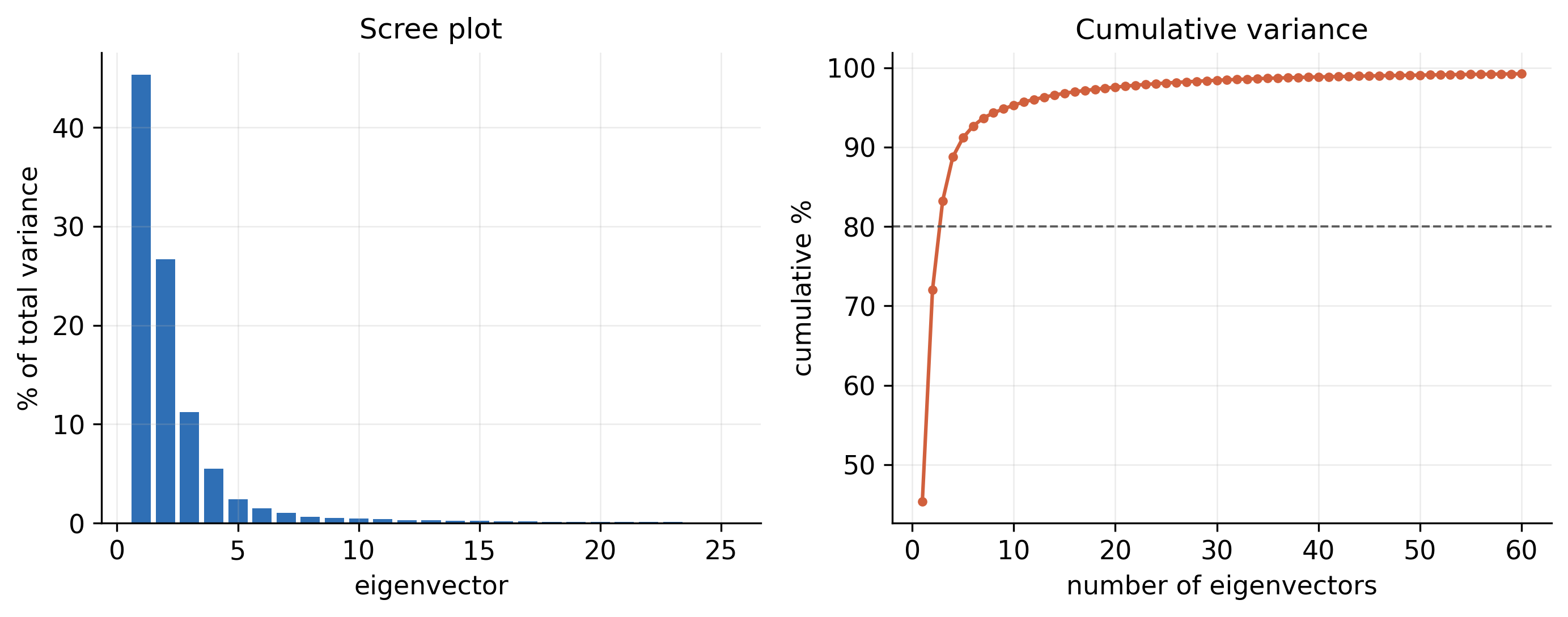
72.0%Motion in the first two principal components

Protein–ligand projects

Binding, not just stability

Most simulation projects are a protein with a drug candidate or phytochemical. On top of the graphs below, protein–ligand projects receive:

01
Ligand RMSD
Whether the ligand stays in the pocket for the whole run, fitted to the protein backbone.
02
Contacts and hydrogen bonds
Which residues hold the ligand, and for what fraction of the simulation.
03
MM-PBSA and MM-GBSA binding free energy
ΔG_bind split into van der Waals, electrostatic, polar and non-polar solvation terms.
04
Per-residue energy decomposition
The pocket residues that contribute most to binding.

The written report

Written for your manuscript

Every project comes with methods and results you can adapt for your paper. These excerpts, lightly shortened, are from the report of the run on this page.

From the methods

All-atom molecular dynamics was performed with GROMACS 2026.3 using the CHARMM36m force field and the CHARMM-modified TIP3P water model. The protein was placed in a dodecahedral box with a minimum solute–wall distance of 1.2 nm, solvated, and neutralised with 0.15 M NaCl. The system was energy-minimised by steepest descent, then equilibrated for 200 ps in the NVT ensemble and 500 ps in the NPT ensemble with position restraints on the protein heavy atoms. Production dynamics were run for 100 ns in the NPT ensemble at 310 K (V-rescale thermostat) and 1 bar (C-rescale barostat) with a 2 fs time step.

From the results

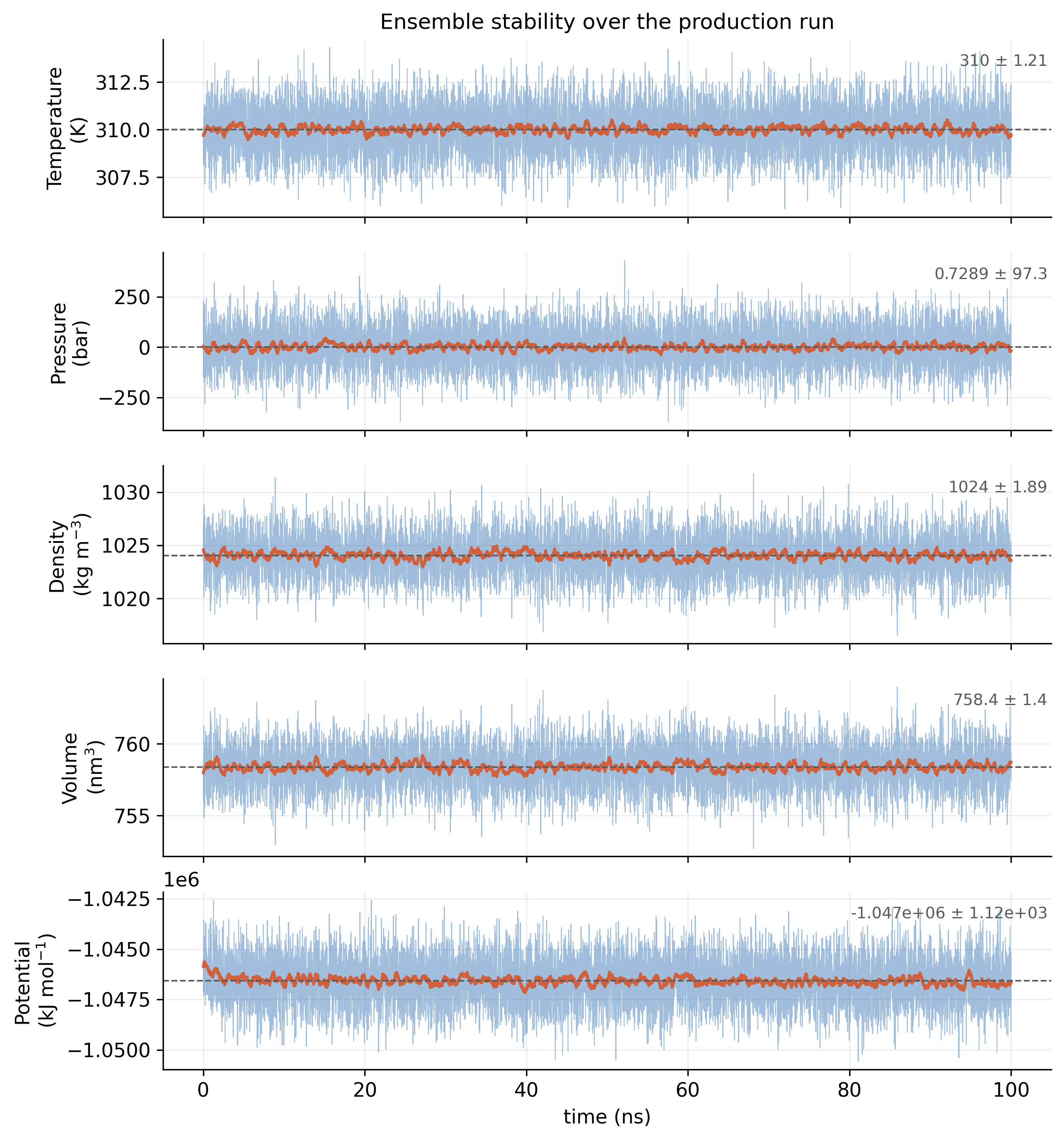
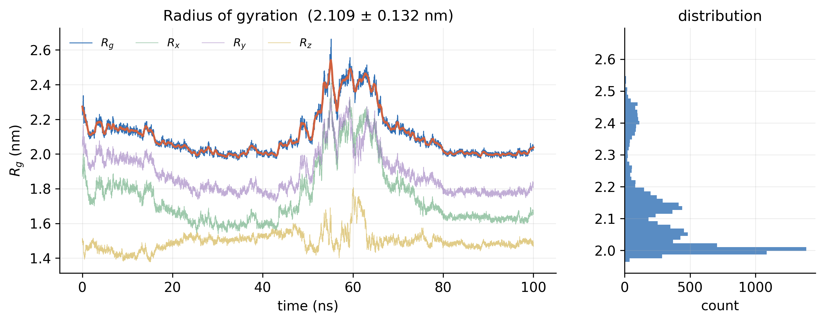
The temperature averaged 310.0 K and the density 1024.1 kg/m³ with no systematic drift. Backbone RMSD relative to the equilibrated structure plateaued at 1.222 ± 0.347 nm, and the radius of gyration remained at 2.109 ± 0.132 nm, indicating that the fold neither unfolded nor collapsed. Principal component analysis showed that the first two eigenvectors accounted for 72.0% of the total fluctuation; the free-energy landscape projected onto them displayed a dominant basin with limited conformational spread.

The system and the run

What was simulated, and was the simulation itself sound?

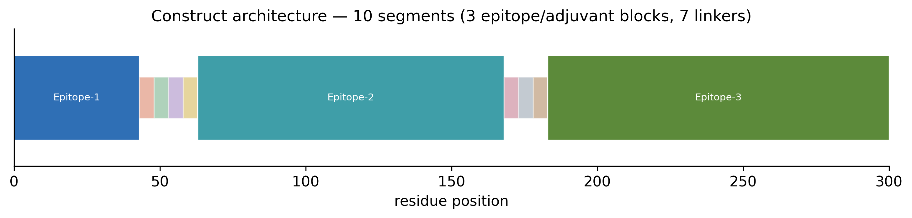
Bar diagram of the construct along residues 1 to 300, showing three epitope blocks separated by short linker segments — Fig. 1Construct architecture. The 300-residue vaccine construct: three epitope blocks joined by seven linkers. PDF

Five stacked time series over 100 ns for temperature, pressure, density, volume and potential energy, each flat around its mean — Fig. 2Ensemble checks. Temperature, pressure, density, volume and potential energy across the production run. Temperature held at 310 K and density at 1024 kg/m³, with no drift. PDF

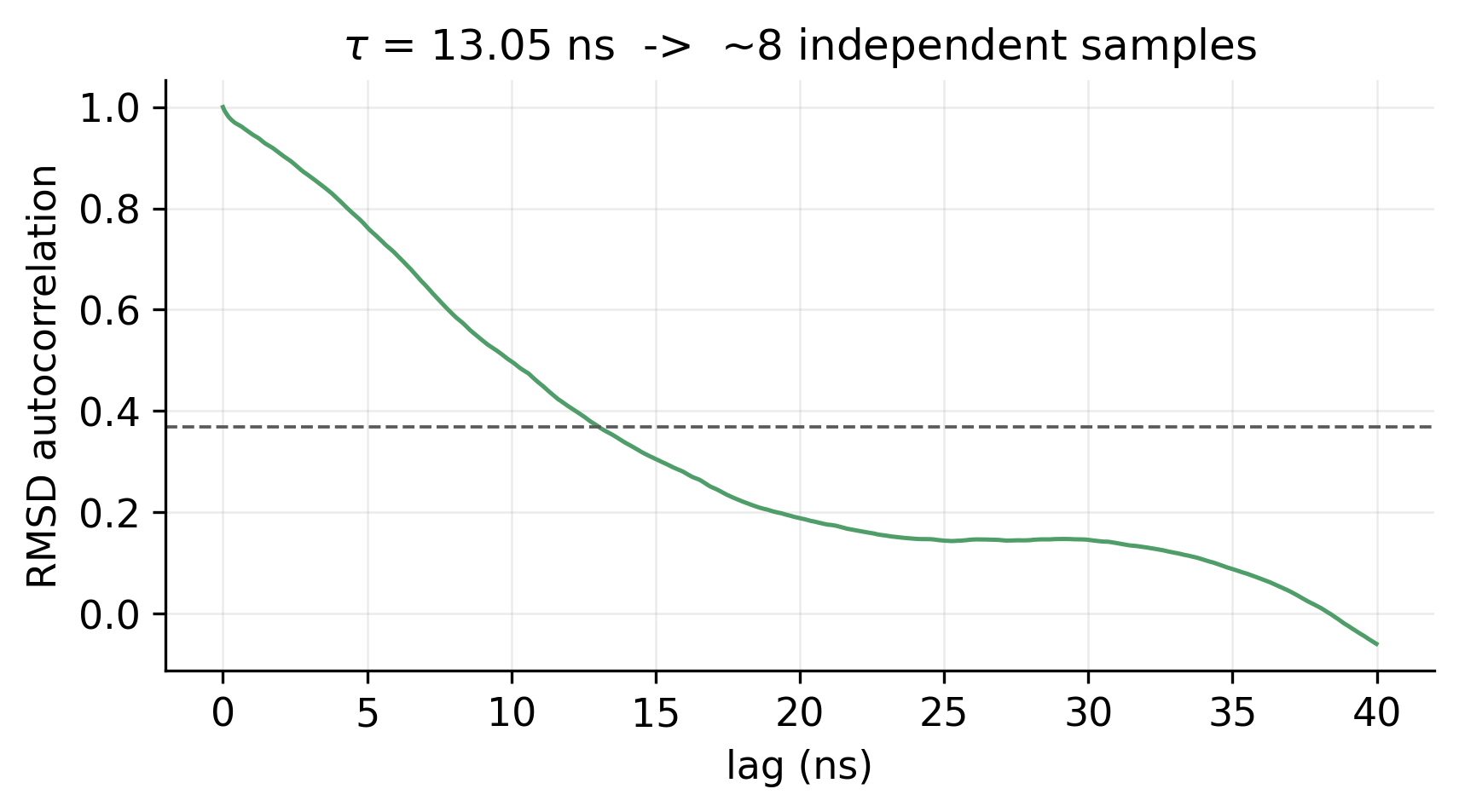
Autocorrelation of RMSD against lag time, falling below the 1/e line at 13 ns — Fig. 3RMSD autocorrelation. A correlation time of 13 ns, which gives about eight statistically independent samples from the run. PDF

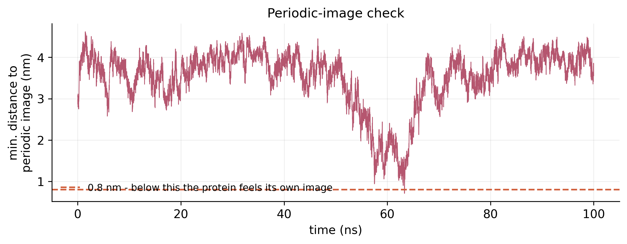
Minimum distance to the nearest periodic image over 100 ns, mostly between 3 and 4 nm with a dip near 62 ns — Fig. 4Periodic-image check. The shortest distance between the protein and its own periodic image at every frame; the lowest point was 0.71 nm, near 62 ns. PDF

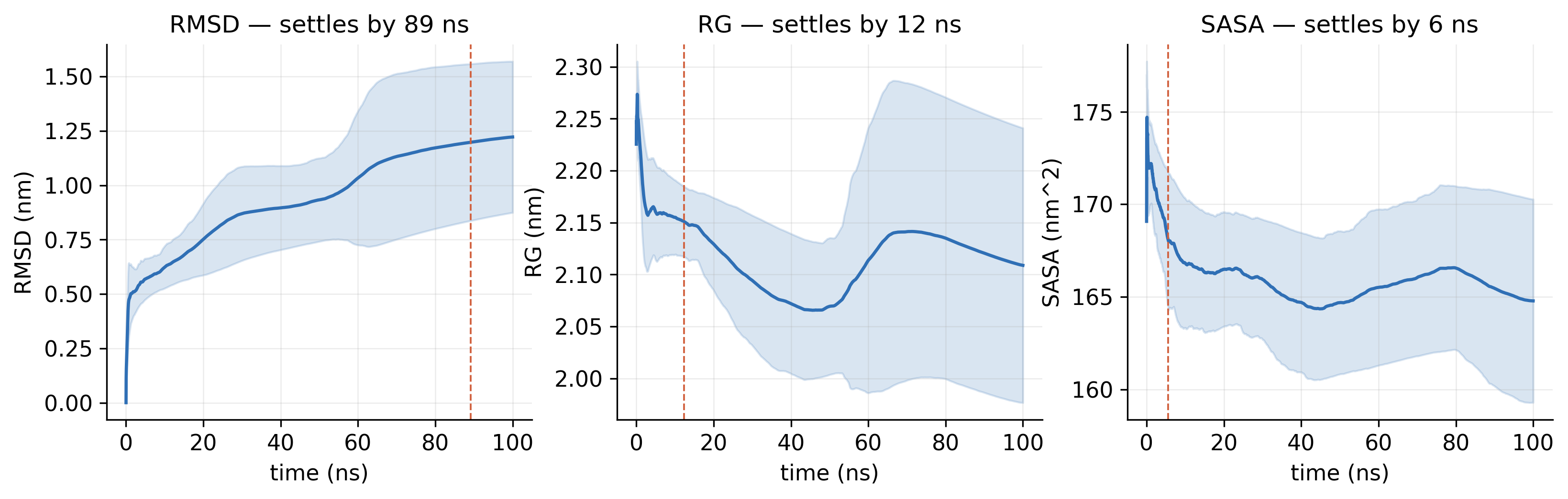
Three panels of running averages with confidence bands for RMSD, radius of gyration and SASA, each marked with its settling time — Fig. 5Running convergence. Running averages of RMSD, radius of gyration and SASA, with the time at which each settles. PDF

Stability and flexibility

Did the structure hold its fold, and which parts move most?

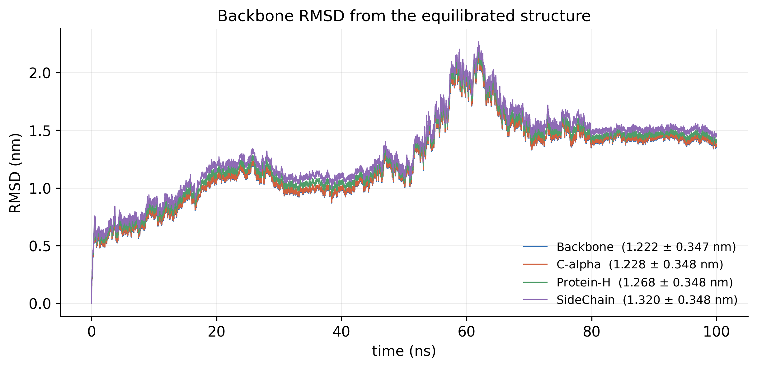
RMSD over 100 ns for backbone, C-alpha, heavy atoms and side chains, rising to a peak near 60 ns and levelling at about 1.4 nm — Fig. 6Backbone RMSD. Deviation from the equilibrated structure, 1.22 ± 0.35 nm on average, with a transition near 60 ns before a plateau from 70 ns. PDF

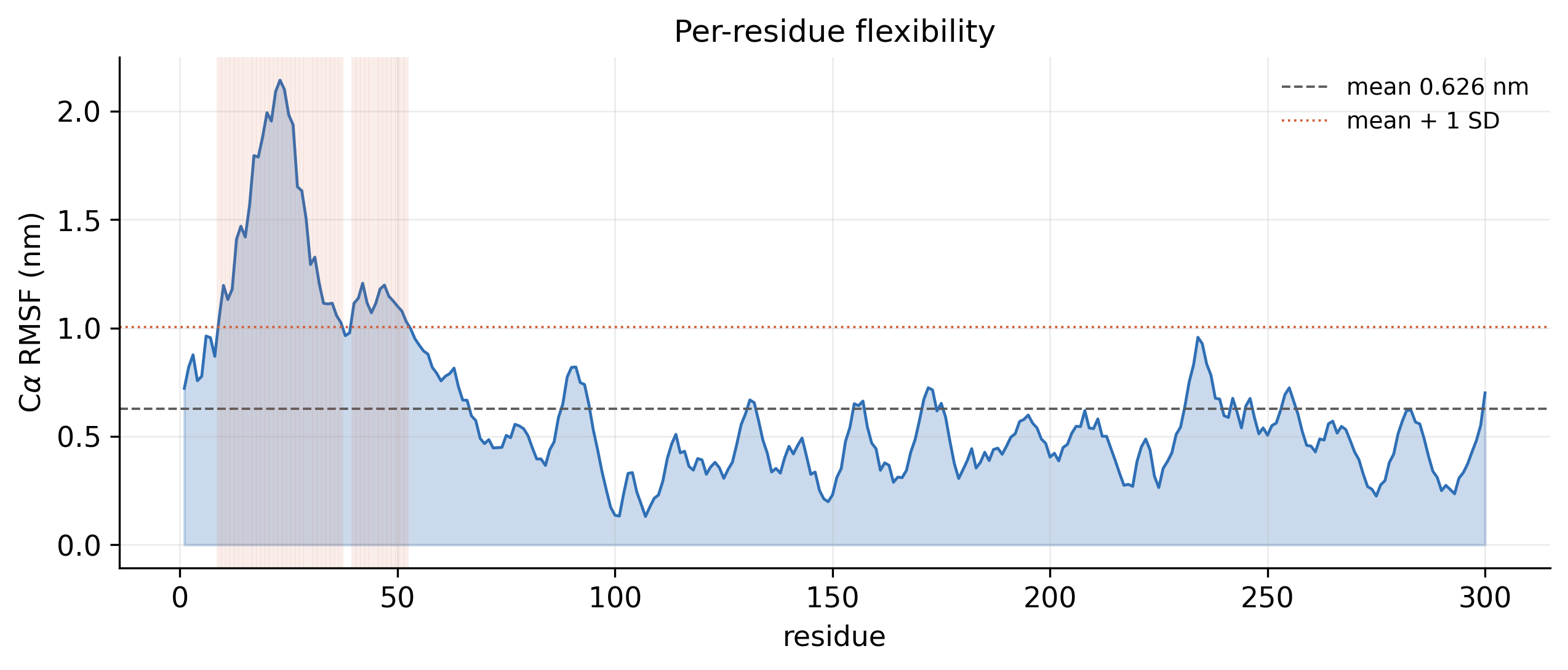
RMSF against residue number with a high peak in the first 50 residues and lower fluctuations elsewhere — Fig. 7Per-residue flexibility (RMSF). C-alpha fluctuation of every residue, 0.63 nm on average; the most flexible region is at the N-terminus. PDF

Radius of gyration and its x, y and z components over 100 ns, with a histogram of values on the right — Fig. 8Radius of gyration. Compactness over time, 2.11 ± 0.13 nm, with its distribution: the fold neither unfolded nor collapsed. PDF

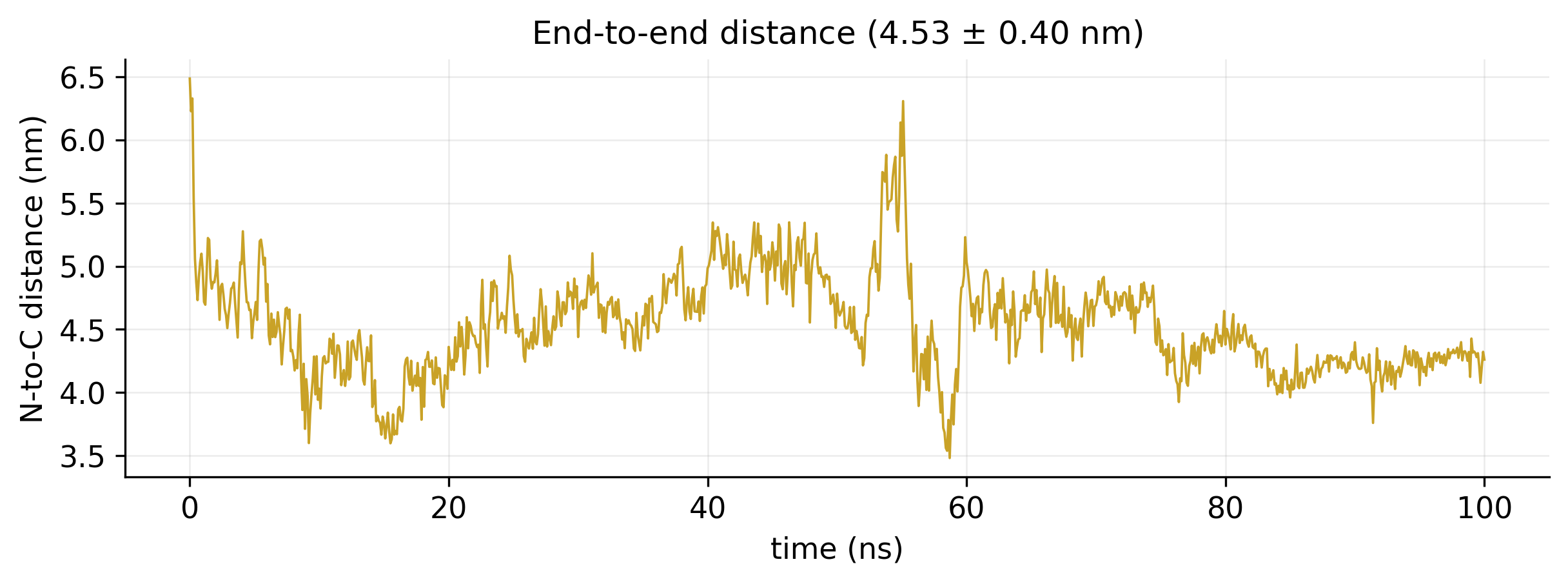
Distance between the two termini over 100 ns, varying between about 3.5 and 6.5 nm — Fig. 9End-to-end distance. Distance between the N- and C-termini, 4.53 ± 0.40 nm. PDF

Structure and contacts

Which structural elements were kept, and which interactions hold them together?

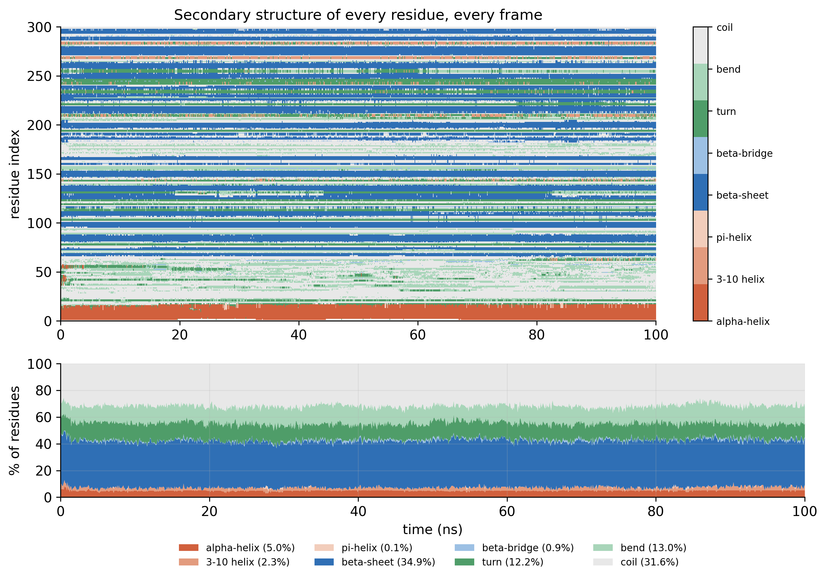
DSSP map of secondary structure per residue over time, with a stacked area chart of percentages below — Fig. 10Secondary structure (DSSP). The state of every residue in every frame: 34.9% beta-sheet and 5.0% helix on average. PDF

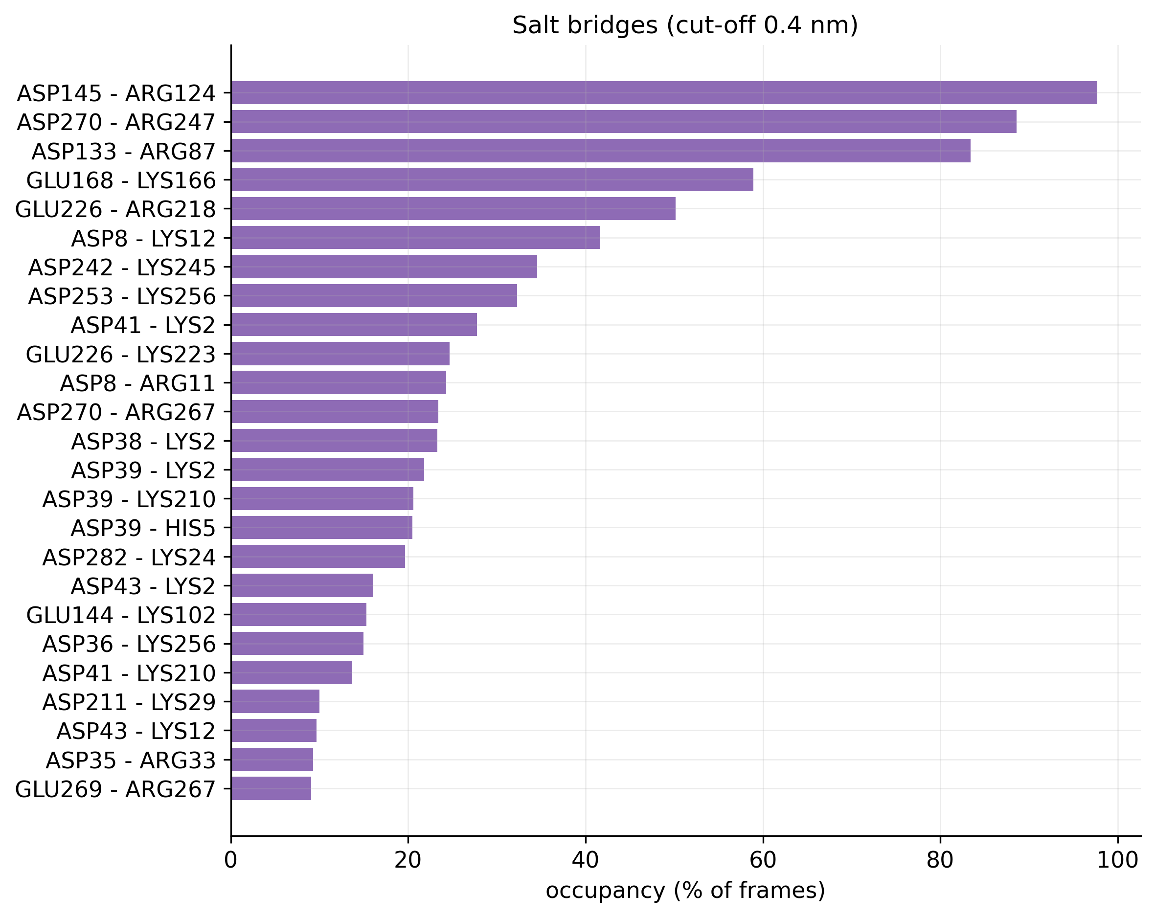
Horizontal bar chart of salt-bridge occupancy, led by ASP145 to ARG124 at nearly 100 percent — Fig. 11Salt bridges. Occupancy of every salt bridge; five are present in more than half of the frames. PDF

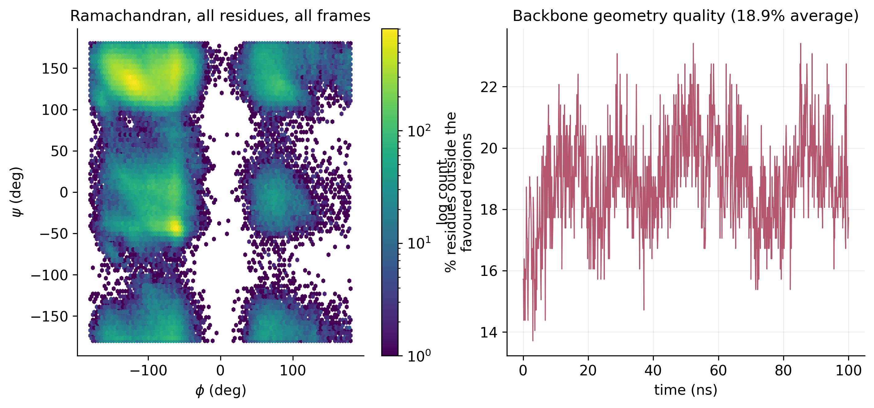
Ramachandran density plot of phi against psi angles, and a time series of the percentage of residues outside favoured regions — Fig. 12Ramachandran plot. Backbone phi and psi angles for all residues across all frames, with the share outside the favoured regions over time. PDF

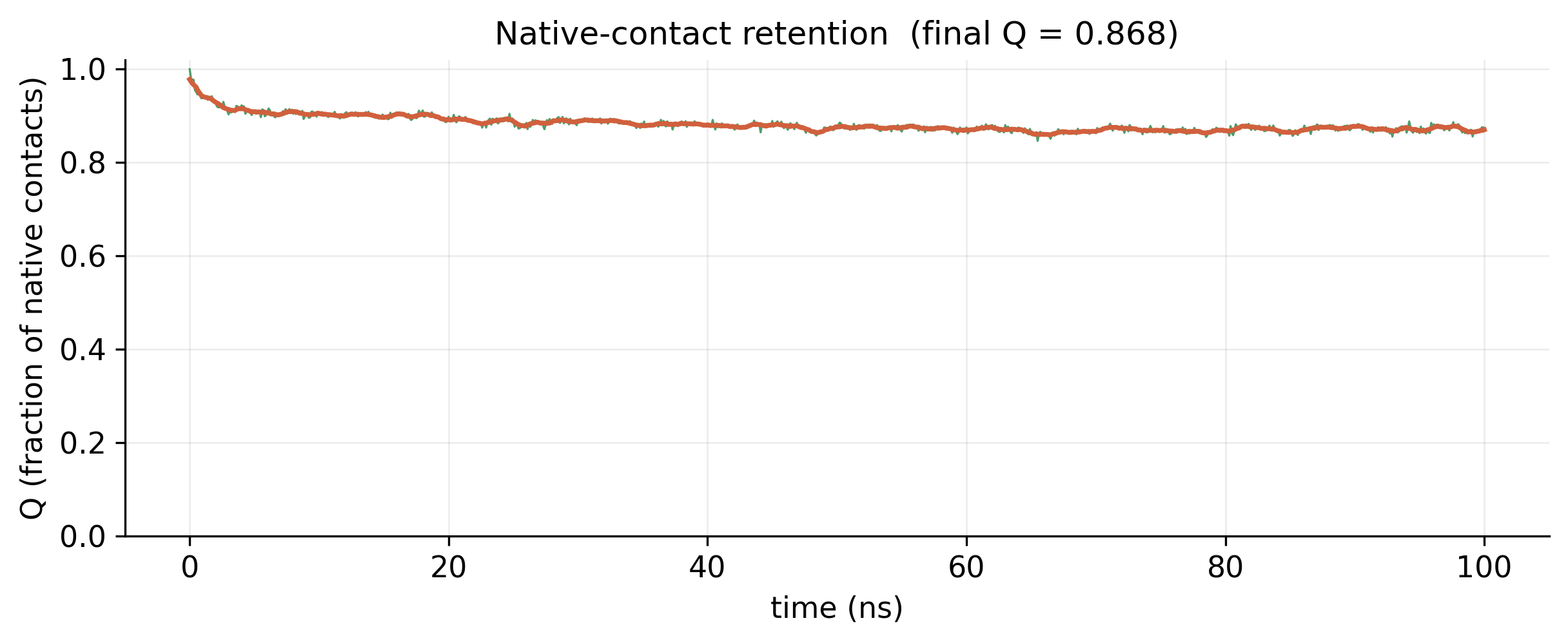
Fraction of native contacts over 100 ns, starting at 1.0 and settling near 0.87 — Fig. 13Native-contact retention. 87% of the starting contacts were still present at 100 ns (Q = 0.868). PDF

Surface and solvent

How much of the protein faces the water, and how does it interact with it?

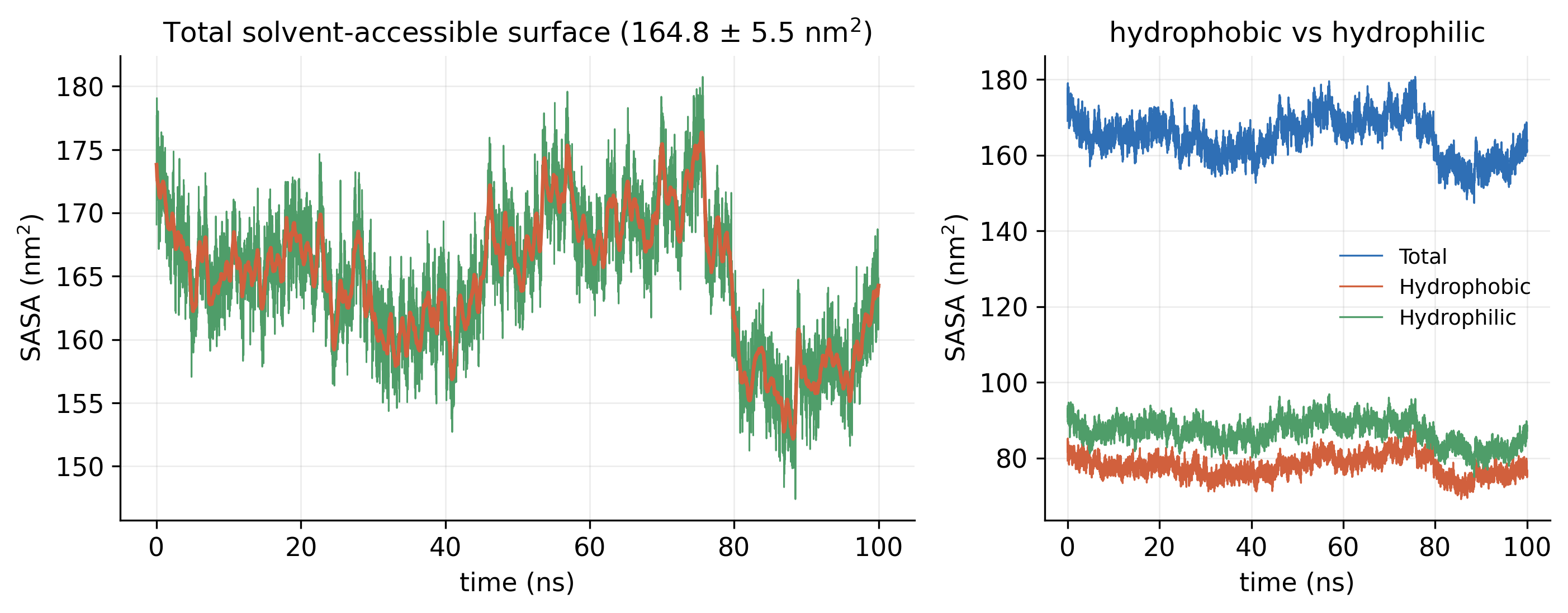
Total SASA over 100 ns, and a second panel splitting it into hydrophobic and hydrophilic surface — Fig. 14Solvent-accessible surface (SASA). Total SASA of 164.8 ± 5.5 nm², split into its hydrophobic and hydrophilic parts. PDF

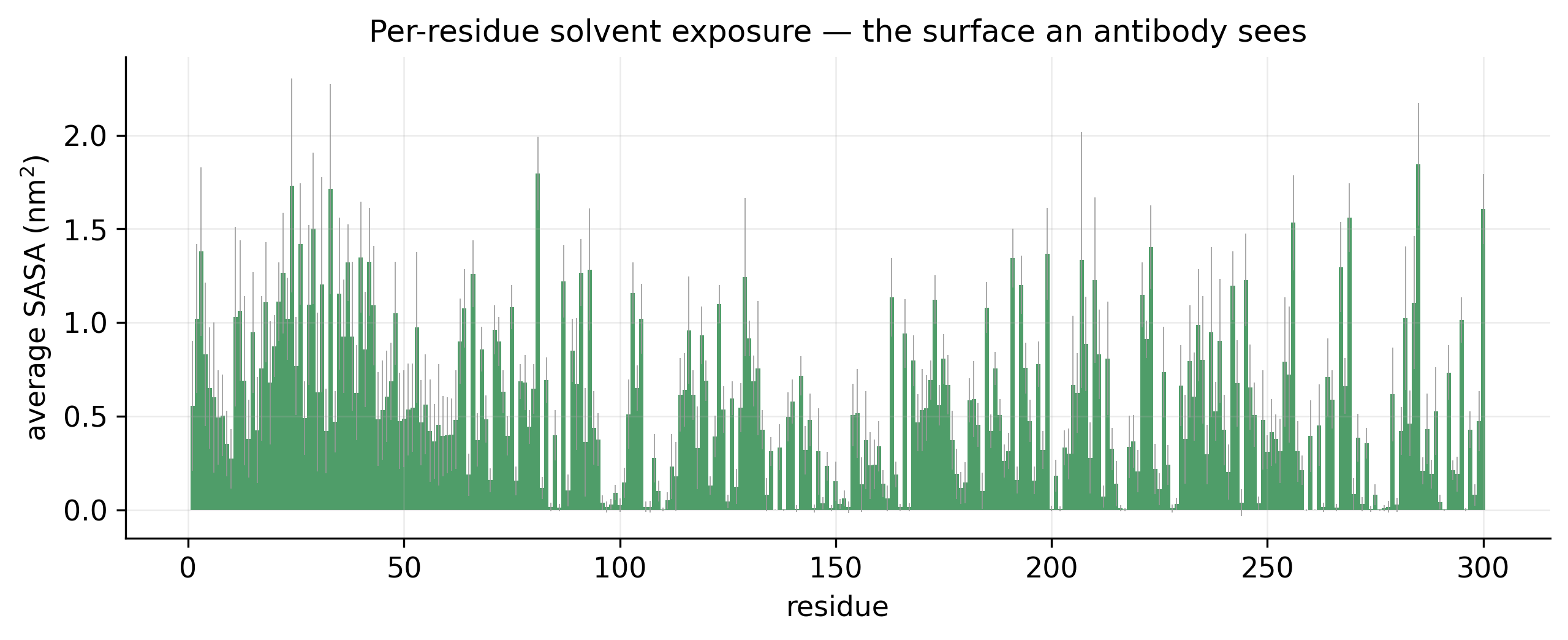
Bar chart of average solvent-accessible surface for each of the 300 residues — Fig. 15Per-residue exposure. Average solvent exposure of each residue: the surface an antibody would see. PDF

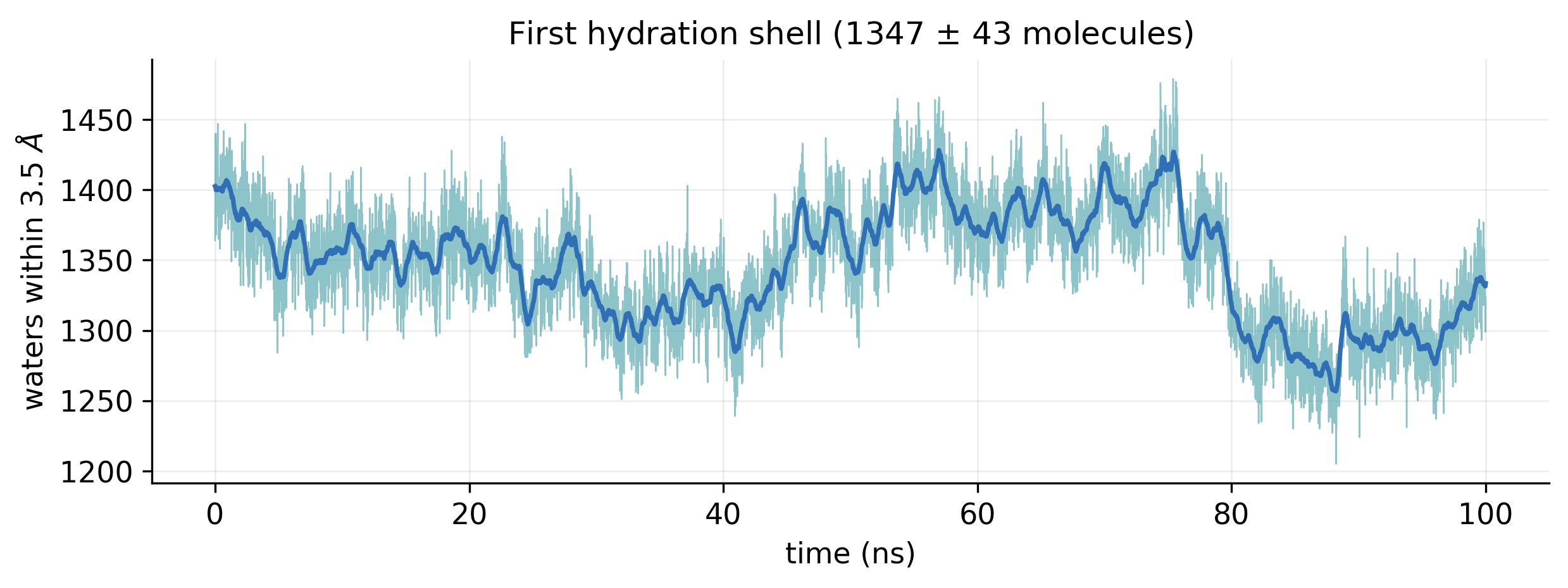
Number of water molecules within 3.5 angstrom of the protein over 100 ns, between about 1250 and 1450 — Fig. 16First hydration shell. Water molecules within 3.5 Å of the protein, 1347 ± 43 on average. PDF

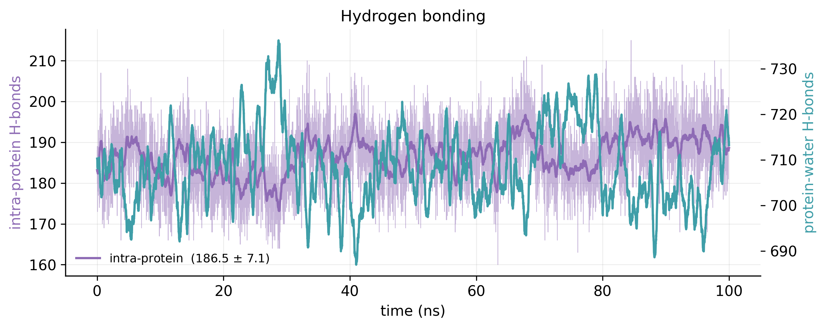
Intra-protein and protein-water hydrogen-bond counts over 100 ns on two axes — Fig. 17Hydrogen bonds. Intra-protein hydrogen bonds (186.5 ± 7.1) and protein–water hydrogen bonds over the run. PDF

Correlated motion and PCA

Which regions move together, and what are the dominant motions?

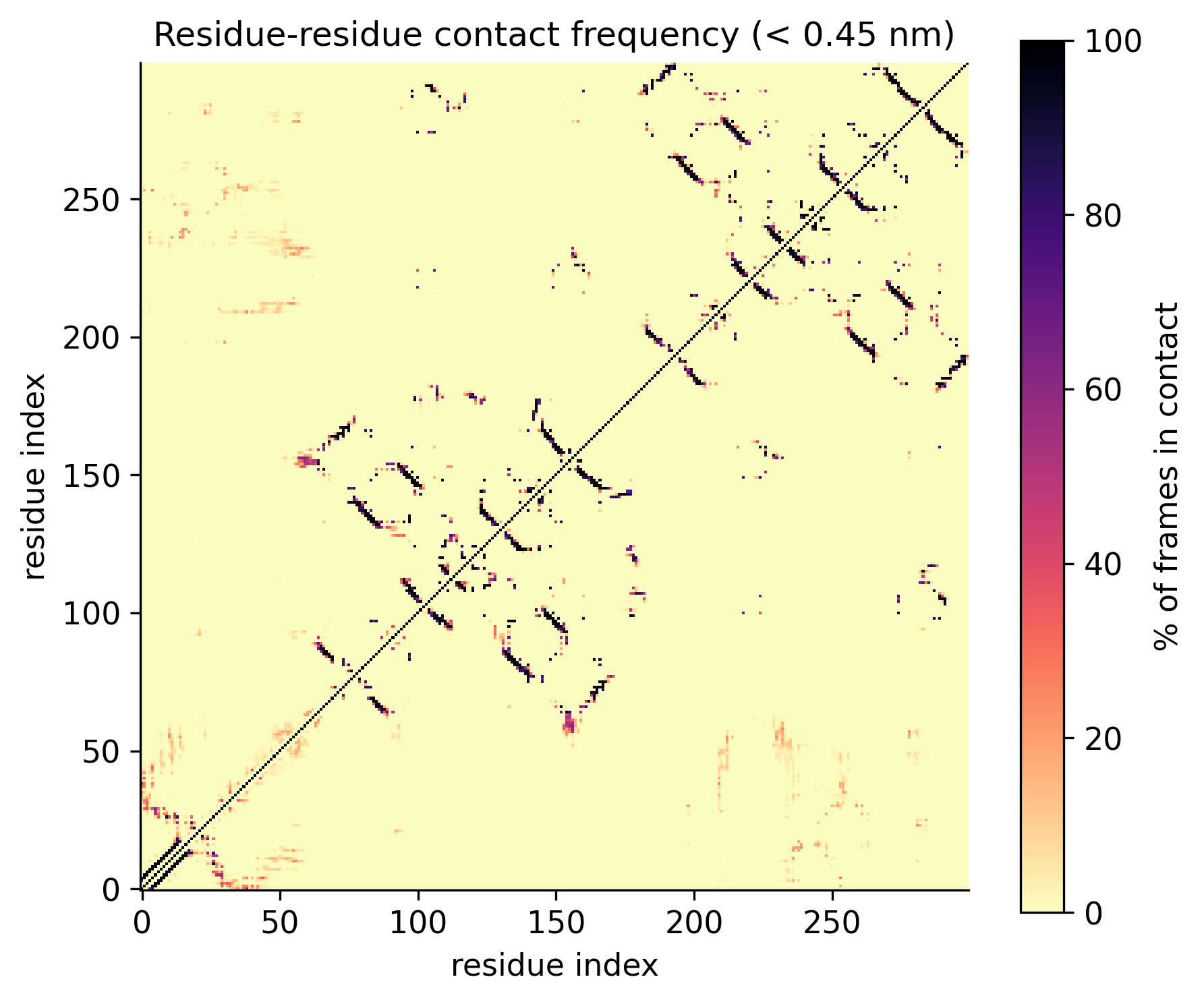
Residue-by-residue contact frequency map showing the diagonal and off-diagonal beta-sheet pairings — Fig. 18Contact map. How often each pair of residues is within 0.45 nm across the run. PDF

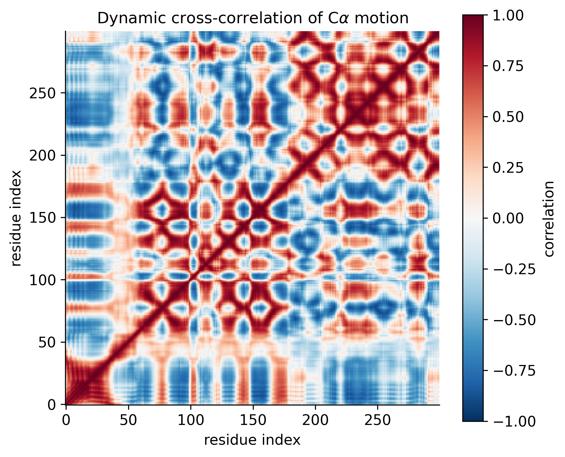
Dynamic cross-correlation matrix of C-alpha motion, red for correlated and blue for anti-correlated pairs — Fig. 19Cross-correlated motion (DCCM). Which regions move together (red) and which move in opposition (blue). PDF

Bar chart of variance per eigenvector and a cumulative variance curve crossing 80 percent at three eigenvectors — Fig. 20PCA scree plot. The first two components carry 72.0% of the motion, and three components reach 80%. PDF

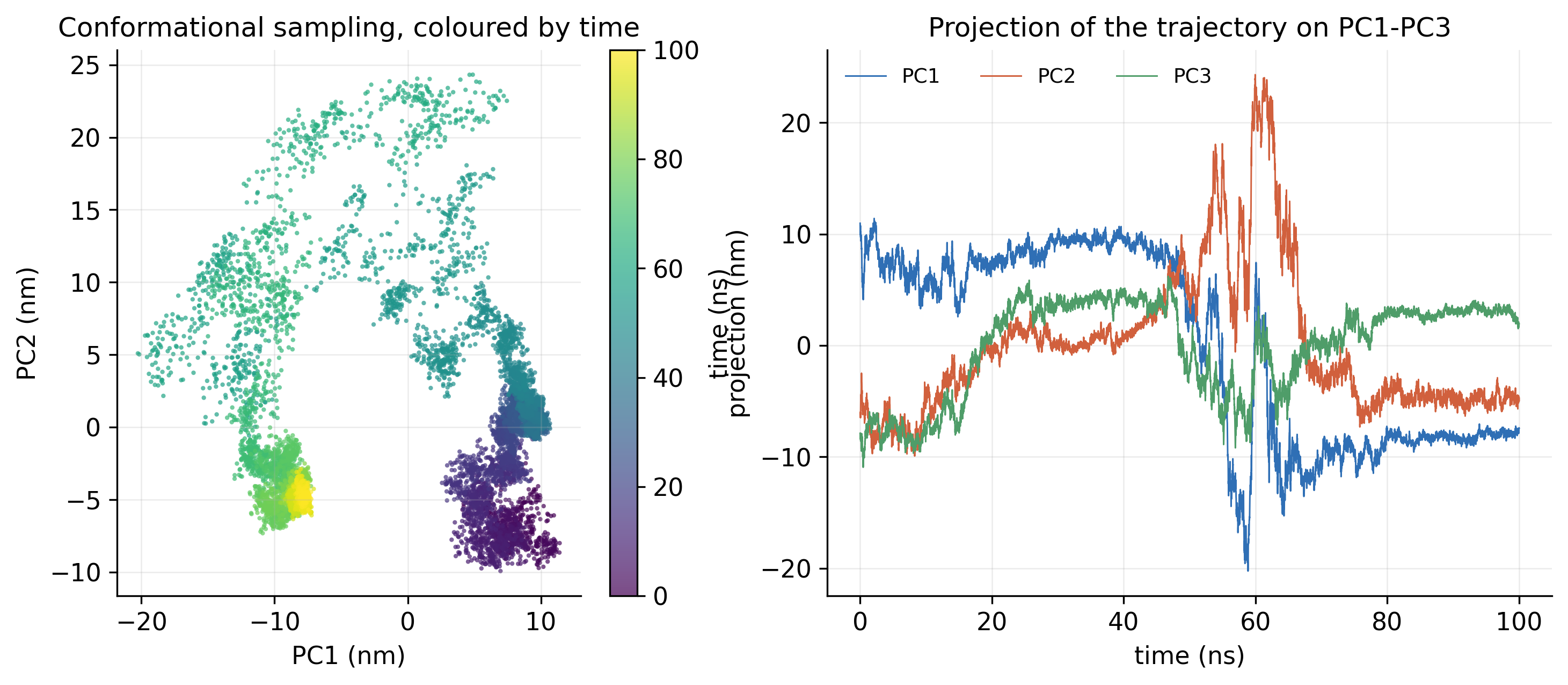
Scatter plot of frames on PC1 against PC2 coloured by time, and time series of PC1, PC2 and PC3 — Fig. 21PCA projection. The trajectory on PC1 and PC2, coloured by time, and its projection on PC1 to PC3 over the run. PDF

Free-energy landscapes

Which conformations does the protein prefer?

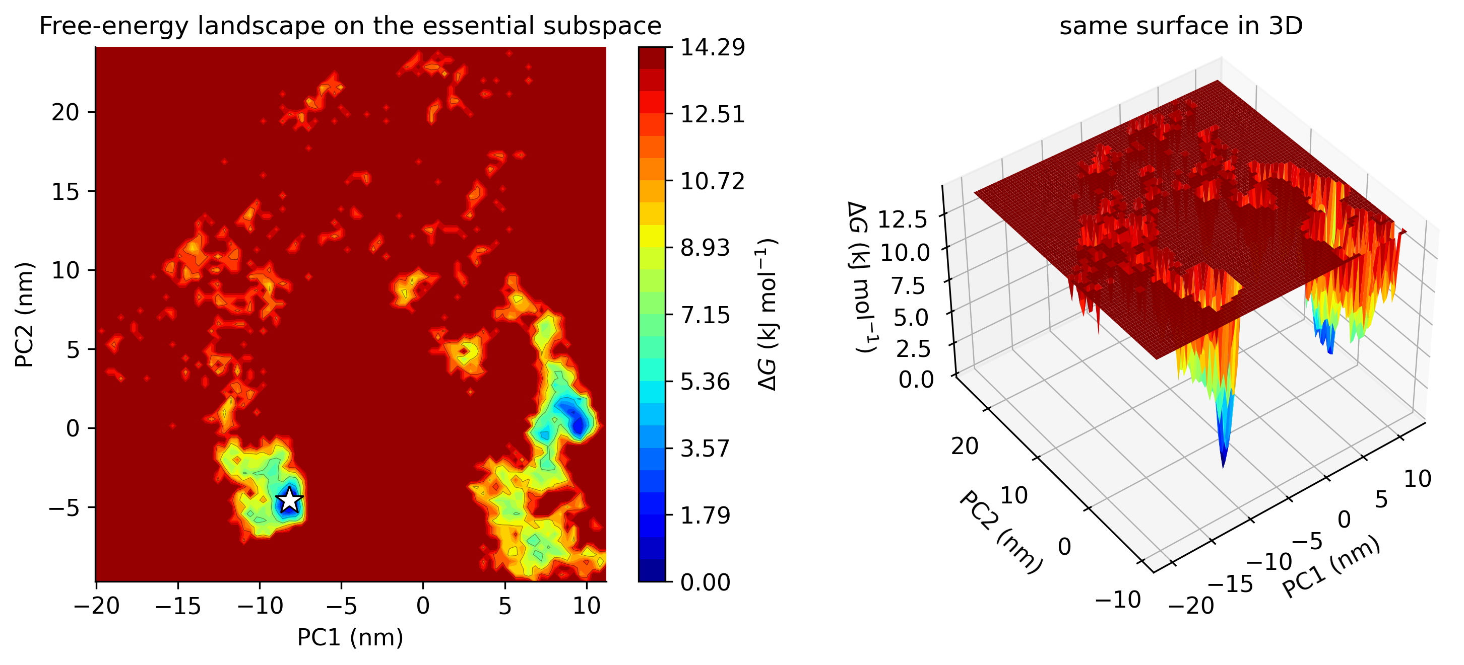
Free-energy landscape on PC1 and PC2 as a contour map and as a 3D surface, with deep blue minima — Fig. 22Free-energy landscape on PC1 and PC2. Gibbs free energy over the first two components, in 2D and 3D; the star marks the lowest-energy state. PDF

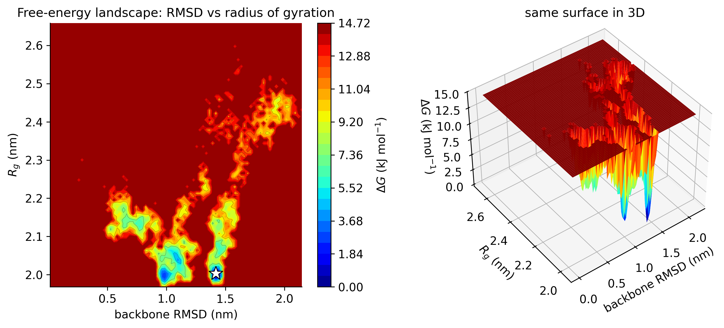
Free-energy landscape of backbone RMSD against radius of gyration as a contour map and as a 3D surface — Fig. 23Free-energy landscape on RMSD and Rg. Gibbs free energy against backbone RMSD and radius of gyration, in 2D and 3D. PDF

You receive

Trajectories and topologies, every graph as an image and an xmgrace file, structure snapshots at chosen time points, a trajectory movie and a written report.

Click any graph to open it at full resolution, or use the PDF link for print. Up to ten simulations run in parallel, so multi-system studies arrive sooner.

Want this analysis for your system?

Send a simulation brief simulations@bioinfoxlab.org